Intro to {biostatR}

(And a Few R Markdown/Quarto Tips!)

Karissa Whiting
Research Biostatistician
Memorial Sloan Kettering

@karissawhiting

github.com/karissawhiting

Agenda

{biostatR}

Intro & Installation
Component Packages
- {gtsummary}
- {lubridate}
- {bstfun}
Extra Features

R Markdown & Quarto

R Markdown Advanced Tips
Quarto

{biostatR}: The ‘tidyverse’ of Analytic Reporting

{biostatR} is a set of packages to help you create and customize analysis reports
Installs and loads 3 useful packages
Also installs (without loading) additional packages to improve your workflow (meaning you’ll need to load these ‘extra packages’ explicitly with library()).

Install {biostatR}

Set up MSK RStudio Package Manager:

Run the following installation code outside of an RStudio project (you only need to do this once!)

install.packages("rstudio.prefs")
rstudio.prefs::use_rstudio_secondary_repo(
  MSK_RSPM = "http://rspm.mskcc.org/MSKREPO/latest"
)

Install {biostatR}

Set up MSK RStudio Package Manager:

Run the following installation code outside of an RStudio project (you only need to do this once!)

install.packages("rstudio.prefs")
rstudio.prefs::use_rstudio_secondary_repo(
  MSK_RSPM = "http://rspm.mskcc.org/MSKREPO/latest"
)

Install {biostatR} From RSPM

install.packages("renv")
renv::install(c("biostatR"))

Three Main Component Packages

{gtsummary} - Tools for creating publication-ready statistical summary tables

Three Main Component Packages

{gtsummary} - Tools for creating publication-ready statistical summary tables
{bstfun} - A miscellaneous collection of functions for our department

Three Main Component Packages

{gtsummary} - Tools for creating publication-ready statistical summary tables
{bstfun} - A miscellaneous collection of functions for our department
{lubridate} - Tools to work with date-times in R

{gtsummary} overview

Create tabular summaries including:
- “Table 1”
- Cross-tabulation
- Regression models summaries
- Survival data summaries
Report statistics from {gtsummary} tables inline in R Markdown
Stack or merge any table type
Use themes to standardize across tables
Choose from different print engines

Basic tbl_summary()

sm_trial <- trial %>% 
  select(trt, age, grade, response)

sm_trial %>%
  select(-trt) %>%
  tbl_summary()

Characteristic	N = 200¹
Age	47 (38, 57)
Unknown	11
Grade
I	68 (34%)
II	68 (34%)
III	64 (32%)
Tumor Response	61 (32%)
Unknown	7
¹ Median (IQR); n (%)

Four types of summaries: continuous, continuous2, categorical, and dichotomous
Variables coded 0/1, TRUE/FALSE, Yes/No treated as dichotomous
Statistics are median (IQR) for continuous, n (%) for categorical/dichotomous
Lists NA values under “Unknown”
Label attributes are printed automatically

Customize tbl_summary() Using Arguments

tbl_summary(
  sm_trial,
  by = trt,
  type = age ~ "continuous2",
  statistic = 
    list(
      age ~ c("{mean} ({sd})", 
              "{min}, {max}"), 
      response ~ "{n} / {N} ({p}%)"
    ),
  label = 
    grade ~ "Pathologic tumor grade",
  digits = age ~ 1
)

Characteristic	Drug A, N = 98¹	Drug B, N = 102¹
Age
Mean (SD)	47.0 (14.7)	47.4 (14.0)
Range	6.0, 78.0	9.0, 83.0
Unknown	7	4
Pathologic tumor grade
I	35 (36%)	33 (32%)
II	32 (33%)	36 (35%)
III	31 (32%)	33 (32%)
Tumor Response	28 / 95 (29%)	33 / 98 (34%)
Unknown	3	4
¹ n (%); n / N (%)

Customize tbl_summary() Using Arguments

tbl_summary(
  sm_trial,
  by = trt,
  type = age ~ "continuous2",
  statistic = 
    list(
      age ~ c("{mean} ({sd})", 
              "{min}, {max}"), 
      response ~ "{n} / {N} ({p}%)"
    ),
  label = 
    grade ~ "Pathologic tumor grade",
  digits = age ~ 1
)

Characteristic	Drug A, N = 98¹	Drug B, N = 102¹
Age
Mean (SD)	47.0 (14.7)	47.4 (14.0)
Range	6.0, 78.0	9.0, 83.0
Unknown	7	4
Pathologic tumor grade
I	35 (36%)	33 (32%)
II	32 (33%)	36 (35%)
III	31 (32%)	33 (32%)
Tumor Response	28 / 95 (29%)	33 / 98 (34%)
Unknown	3	4
¹ n (%); n / N (%)

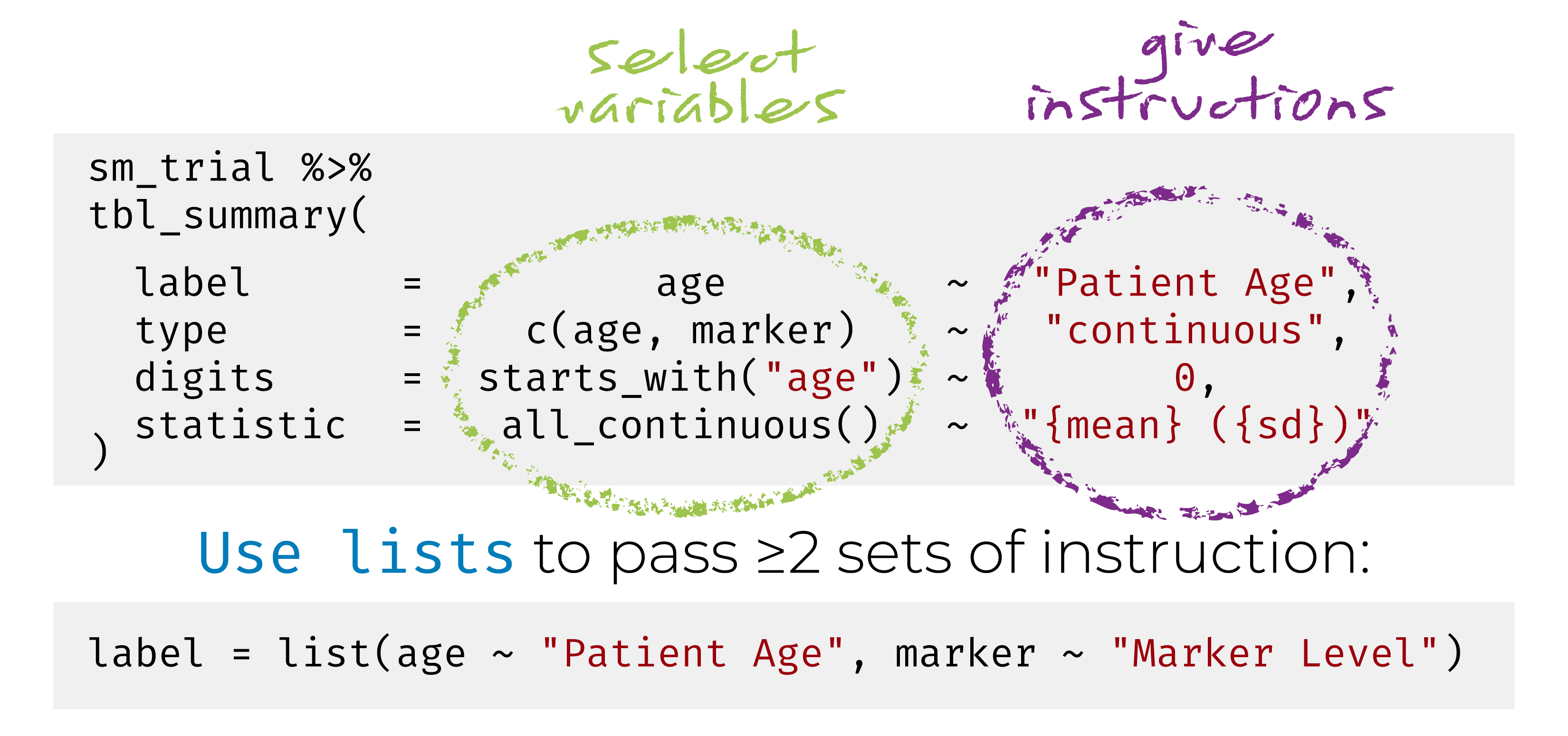
by: specifies a column variable for cross-tabulation
type: specifies the summary type
statistic: customize the reported statistics
label: change or customize variable labels
digits: specify the number of decimal places for rounding

{gtsummary} + formulas

Customize Using Add-on Functions

Summary tables can be further updated using helper functions:

add_*() add additional column of statistics or information, e.g. p-values, q-values, overall statistics, treatment differences, N obs., and more
modify_*() modify table headers, spanning headers, footnotes, and more
bold_()/italicize_() style labels, variable levels, significant p-values

Update tbl_summary() with add_*()

sm_trial %>%
  tbl_summary(
    by = trt
  ) %>% 
  add_p() %>% 
  add_q(method = "fdr")

Characteristic	Drug A, N = 98¹	Drug B, N = 102¹	p-value²	q-value³
Age	46 (37, 59)	48 (39, 56)	0.7	0.9
Unknown	7	4
Grade			0.9	0.9
I	35 (36%)	33 (32%)
II	32 (33%)	36 (35%)
III	31 (32%)	33 (32%)
Tumor Response	28 (29%)	33 (34%)	0.5	0.9
Unknown	3	4
¹ Median (IQR); n (%)
² Wilcoxon rank sum test; Pearson’s Chi-squared test
³ False discovery rate correction for multiple testing

add_p(): adds a column of p-values
add_q(): adds a column of p-values adjusted for multiple comparisons through a call to p.adjust()

Update tbl_summary() with add_*()

sm_trial %>%
  tbl_summary(
    by = trt,
    missing = "no"
  ) %>% 
  add_overall() %>% 
  add_n() %>% 
  add_stat_label(
    label = all_categorical() ~ "No. (%)"
  )

Characteristic	N	Overall, N = 200	Drug A, N = 98	Drug B, N = 102
Age, Median (IQR)	189	47 (38, 57)	46 (37, 59)	48 (39, 56)
Grade, No. (%)	200
I		68 (34%)	35 (36%)	33 (32%)
II		68 (34%)	32 (33%)	36 (35%)
III		64 (32%)	31 (32%)	33 (32%)
Tumor Response, No. (%)	193	61 (32%)	28 (29%)	33 (34%)

add_overall(): adds a column of overall statistics
add_n(): adds a column with the sample size
add_stat_label(): adds a description of the reported statistic

Update with bold_() or italicize_()

sm_trial %>%
  tbl_summary(
    by = trt
  ) %>%
  add_p() %>% 
  bold_labels() %>% 
  italicize_levels() %>% 
  bold_p(t = 0.8)

Characteristic	Drug A, N = 98¹	Drug B, N = 102¹	p-value²
Age	46 (37, 59)	48 (39, 56)	0.7
Unknown	7	4
Grade			0.9
I	35 (36%)	33 (32%)
II	32 (33%)	36 (35%)
III	31 (32%)	33 (32%)
Tumor Response	28 (29%)	33 (34%)	0.5
Unknown	3	4
¹ Median (IQR); n (%)
² Wilcoxon rank sum test; Pearson’s Chi-squared test

bold_labels(): bold the variable labels
italicize_levels(): italicize the variable levels
bold_p(): bold p-values according a specified threshold

Update tbl_summary() with modify_*()

sm_trial %>% 
  tbl_summary(
    by = trt, missing = "no"
  ) %>%
  modify_header(
      stat_1 ~ "**Group A**",
      stat_2 ~ "**Group B**"
  ) %>% 
  modify_spanning_header(
    all_stat_cols() ~ "**Drug**") %>% 
  modify_footnote(
    all_stat_cols() ~ 
      paste("median (IQR) for continuous;",
            "n (%) for categorical")
  )

Characteristic	Drug
Characteristic	Group A¹	Group B¹
Age	46 (37, 59)	48 (39, 56)
Grade
I	35 (36%)	33 (32%)
II	32 (33%)	36 (35%)
III	31 (32%)	33 (32%)
Tumor Response	28 (29%)	33 (34%)
¹ median (IQR) for continuous; n (%) for categorical

Use show_header_names() to see the internal header names available for use in modify_header()

Customize Using Add-on Functions

Many more customization available!

See the documentation at http://www.danieldsjoberg.com/gtsummary/reference/index.html

And a detailed tbl_summary() vignette at http://www.danieldsjoberg.com/gtsummary/articles/tbl_summary.html

Quick Code Exercise

1. Create new data frame (new_trial) and select columns age, stage, response, marker

2. Make a basic tbl_summary() summarizing by response variable and add the following customization:

For age make statistic report the"{mean} ({min}, {max})"
Use missing arg to remove display of missing values

3. Now apply the following customization:

add a p-value
bold labels and p-values ≤ .05, italicize levels
add an ‘overall’ column

See documentation for help: https://www.danieldsjoberg.com/gtsummary/

Quick Code Exercise

1. Create new data frame (new_trial) and select columns age, stage, response, marker

2. Make a basic tbl_summary() summarizing by response variable and add the following customization:

For age make statistic report the"{mean} ({min}, {max})"
Use missing arg to remove display of missing values

3. Now apply the following customization:

add a p-value
bold labels and p-values ≤ .05, italicize levels
add an ‘overall’ column

new_trial <- select(trial, age, stage, response, marker)

Quick Code Exercise

1. Create new data frame (new_trial) and select columns age, stage, response, marker

2. Make a basic tbl_summary() summarizing by response variable and add the following customization:

For age make statistic report the"{mean} ({min}, {max})"
Use missing arg to remove display of missing values

3. Now apply the following customization:

add a p-value
bold labels and p-values ≤ .05, italicize levels
add an ‘overall’ column

new_trial <- select(trial, age, stage, response, marker)

new_trial %>%
  tbl_summary(by = response, 
              statistic = age ~ "{mean} ({min}, {max})", 
              missing = "no")

Characteristic	0, N = 132¹	1, N = 61¹
Age	46 (6, 83)	50 (9, 78)
T Stage
T1	34 (26%)	18 (30%)
T2	39 (30%)	13 (21%)
T3	25 (19%)	15 (25%)
T4	34 (26%)	15 (25%)
Marker Level (ng/mL)	0.59 (0.21, 1.24)	0.98 (0.31, 1.53)
¹ Mean (Range); n (%); Median (IQR)

Quick Code Exercise

1. Create new data frame (new_trial) and select columns age, stage, response, marker

2. Make a basic tbl_summary() summarizing by response variable and add the following customization:

For age make statistic report the"{mean} ({min}, {max})"
Use missing arg to remove display of missing values

3. Now apply the following customization:

add a p-value
bold labels and p-values ≤ .05, italicize levels
add an ‘overall’ column

new_trial <- select(trial, age, stage, response, marker)

new_trial %>%
  tbl_summary(by = response, 
              statistic = age ~ "{mean} ({min}, {max})", 
              missing = "no") %>%
  add_p() %>%
  bold_labels() %>%
  bold_p() %>%
  italicize_levels() %>%
  add_overall()

Characteristic	Overall, N = 193¹	0, N = 132¹	1, N = 61¹	p-value²
Age	47 (6, 83)	46 (6, 83)	50 (9, 78)	0.091
T Stage				0.6
T1	52 (27%)	34 (26%)	18 (30%)
T2	52 (27%)	39 (30%)	13 (21%)
T3	40 (21%)	25 (19%)	15 (25%)
T4	49 (25%)	34 (26%)	15 (25%)
Marker Level (ng/mL)	0.62 (0.22, 1.38)	0.59 (0.21, 1.24)	0.98 (0.31, 1.53)	0.10
¹ Mean (Range); n (%); Median (IQR)
² Wilcoxon rank sum test; Pearson’s Chi-squared test

Survival outcomes with tbl_survfit()

library(survival)
fit <- survfit(Surv(ttdeath, death) ~ trt, trial)
tbl_survfit(
  fit, 
  times = c(12, 24),
  label_header = "**{time} Month**"
) %>%
  add_p()

Characteristic	12 Month	24 Month	p-value¹
Chemotherapy Treatment			0.2
Drug A	91% (85%, 97%)	47% (38%, 58%)
Drug B	86% (80%, 93%)	41% (33%, 52%)
¹ Log-rank test

Model Summaries with tbl_regression()

m1 <- glm(
  response ~ age + stage,
  data = trial,
  family = binomial(link = "logit")
  )


tbl_regression(
    m1,
    exponentiate = TRUE
  ) %>% 
  add_global_p()

Characteristic	OR¹	95% CI¹	p-value
Age	1.02	1.00, 1.04	0.087
T Stage			0.6
T1	—	—
T2	0.58	0.24, 1.37
T3	0.94	0.39, 2.28
T4	0.79	0.33, 1.90
¹ OR = Odds Ratio, CI = Confidence Interval

Univariate models with tbl_uvregression()

tbl_uvreg <- sm_trial %>% 
  tbl_uvregression(
    method = glm,
    y = response,
    method.args = list(family = binomial),
    exponentiate = TRUE
  ) %>%
  bold_labels()

tbl_uvreg

Characteristic	N	OR¹	95% CI¹	p-value
Chemotherapy Treatment	193
Drug A		—	—
Drug B		1.21	0.66, 2.24	0.5
Age	183	1.02	1.00, 1.04	0.10
Grade	193
I		—	—
II		0.95	0.45, 2.00	0.9
III		1.10	0.52, 2.29	0.8
¹ OR = Odds Ratio, CI = Confidence Interval

Specify model method, method.args, and the response variable
Arguments and helper functions like exponentiate, bold_*(), add_global_p() can also be used with tbl_uvregression()

{bstfun}

A shared space for department members to add functions that may be useful to others
Houses individual member’s project templates and function to start projects (create_bst_project(): will be discussed in further training)
Diverse functions for various analysis-related tasks, {bstfun} Reference Index: https://www.danieldsjoberg.com/bstfun/reference/index.html

{bstfun} Useful Functions

style_tbl_compact()

Before:

head(trial) %>%
  gt::gt() %>%
  bstfun::style_tbl_compact()

trt	age	marker	stage	grade	response	death	ttdeath
Drug A	23	0.160	T1	II	0	0	24.00
Drug B	9	1.107	T2	I	1	0	24.00
Drug A	31	0.277	T1	II	0	0	24.00
Drug A	NA	2.067	T3	III	1	1	17.64
Drug A	51	2.767	T4	III	1	1	16.43
Drug B	39	0.613	T4	I	0	1	15.64

After:

head(trial) %>%
  gt::gt()

trt	age	marker	stage	grade	response	death	ttdeath
Drug A	23	0.160	T1	II	0	0	24.00
Drug B	9	1.107	T2	I	1	0	24.00
Drug A	31	0.277	T1	II	0	0	24.00
Drug A	NA	2.067	T3	III	1	1	17.64
Drug A	51	2.767	T4	III	1	1	16.43
Drug B	39	0.613	T4	I	0	1	15.64

❗ Also see tbl_listing() for this functionality: https://shannonpileggi.github.io/gtreg/reference/tbl_listing.html

{bstfun} Useful Functions

clean_mrn()

MRNs follows specific formatting rules:

Must be character
Must contain only numeric components
Must be eight characters long and include leading zeros.

This function converts numeric MRNs to character and ensures it follows MRN conventions. Character MRNs can also be passed, and leading zeros will be appended and checked for consistency.

fake_mrn <- c("00100", "100", "0100")

fake_mrn %>%
  bstfun::clean_mrn()

[1] “00000100” “00000100” “00000100”

{bstfun} Useful Functions

use_varnames_as_labels()

Automatically add labels to your data based on column names

Before:

mtcars %>%
  select(mpg, cyl, vs, am) %>%
  tbl_summary()

Characteristic	N = 32¹
mpg	19.2 (15.4, 22.8)
cyl
4	11 (34%)
6	7 (22%)
8	14 (44%)
vs	14 (44%)
am	13 (41%)
¹ Median (IQR); n (%)

After:

mtcars %>%
  select(mpg, cyl, vs, am) %>%
  bstfun::use_varnames_as_labels(caps = c(mpg, vs), exclude = cyl) %>%
  tbl_summary()

Characteristic	N = 32¹
MPG	19.2 (15.4, 22.8)
cyl
4	11 (34%)
6	7 (22%)
8	14 (44%)
VS	14 (44%)
Am	13 (41%)
¹ Median (IQR); n (%)

{lubridate}

We work with a LOT of dates
{lubridate} helps parse dates from strings, and improves functional operations on date-times
Data cleaning training will cover this in more depth or see R for Data Science: https://r4ds.had.co.nz/dates-and-times.html

library(lubridate)

bday <- dmy("14/10/1940")
month(bday)

[1] 10

wday(bday, label = TRUE)

[1] Mon Levels: Sun < Mon < Tue < Wed < Thu < Fri < Sat

year(bday) <- 2016
wday(bday, label = TRUE)

[1] Fri Levels: Sun < Mon < Tue < Wed < Thu < Fri < Sat

{biostatR} Bonus Features

When you load {biostatR} it will:
- Check if any packages are out of date
- Check if RSPM is set up
- Check if you are more than 2 versions behind the latest version of R
It also installs some useful dependencies, including:
- {flextable} - Better defaults for knitting Rmd to word documents
- {styler} - Makes your code pretty
- {ragg} - Better graphics printing
- {mskRvis} - MSK color palettes
- {mskRutils} - Helpful functions for working with MSK github

R Markdown Tips

Report Reproducbile Statistics with gtsummary::inline_text()

Tables are important, but we often need to report results in-line in a report.
Any statistic reported in a {gtsummary} table can be extracted and reported in-line in an R Markdown document with the inline_text() function.
The pattern of what is reported can be modified with the pattern = argument.
Default is pattern = "{estimate} ({conf.level*100}% CI {conf.low}, {conf.high}; {p.value})"

Report Reproducbile Statistics with gtsummary::inline_text()

library(gtsummary)

tbl_uvreg <- sm_trial %>% 
  tbl_uvregression(
    method = glm,
    y = response,
    method.args = list(family = binomial),
    exponentiate = TRUE
  ) %>%
  bold_labels()

tbl_uvreg

Characteristic	N	OR¹	95% CI¹	p-value
Chemotherapy Treatment	193
Drug A		—	—
Drug B		1.21	0.66, 2.24	0.5
Age	183	1.02	1.00, 1.04	0.10
Grade	193
I		—	—
II		0.95	0.45, 2.00	0.9
III		1.10	0.52, 2.29	0.8
¹ OR = Odds Ratio, CI = Confidence Interval

In Code: The odds ratio for age is ‘inline_text(tbl_uvreg, variable = age)’

In Report: The odds ratio for age is 1.02 (95% CI 1.00, 1.04; p=0.10)

Add Tabs to Your Report

Quarto

What is Quarto?

Quarto is a multi-language, next generation version of R Markdown from RStudio
Like R Markdown, Quarto uses Knitr to execute R code, therefore it can render most existing Rmd files with few changes
The latest release of RStudio (v2022.07) includes support for editing and preview of Quarto documents.

Quarto Features: Flexible Layouts

You can now easily organize your report using various layouts including column formats

plot(cars)
plot(pressure)

Vapor Pressure of Mercury as a Function of Temperature

Quarto Features

You can execute R and Python code in the same file
Auto-fill YAML options for easy, fool-proof YAML coding
Cleaner organization (e.g. Global chunk options can now go in YAML header)

Moving From R Markdown: YAML Header

YAML Header now uses format instead of output and allows auto-complete to make editing the YAML more fool-proof.

R Markdown:

#| code-line-numbers: "2"

title: "My Document"
output:
  html_document:
    toc: true
    number_sections: true
    css: styles.css

Quarto:

#| code-line-numbers: "2"

title: "My Document"
format:
  html:
    toc: true
    number-sections: true
    css: styles.css

Moving From R Markdown: YAML Header

Global chunk options are set in YAML header using execute instead of in a knitr setup chunk.

R Markdown:

Quarto:

title: "My-Title"
subtitle: "Until now!"
execute:
  echo: false

Moving From R Markdown: YAML Chunk Options

Individual chunk options are also set in YAML in each chunk as needed, using the “hashpipe” (#|).

R Markdown:

Quarto:

Thank You!!!

Questions?

Resources

{biostaR} - https://github.mskcc.org/pages/datadojo/biostatR/index.html
{gtsummary} - https://www.danieldsjoberg.com/gtsummary/
{bstfun} - https://www.danieldsjoberg.com/bstfun/index.html
Departmental Resource Guide - https://rconnect.mskcc.org/resource-guide/
Quarto Docs - https://quarto.org/docs/guide/
Quarto Blog Post by Alison Hill - https://www.apreshill.com/blog/2022-04-we-dont-talk-about-quarto/

Intro to {biostatR}

Agenda

{biostatR}: The ‘tidyverse’ of Analytic Reporting

Install {biostatR}

Install {biostatR}

Install {biostatR}

Three Main Component Packages

Three Main Component Packages

Three Main Component Packages

Three Main Component Packages

{gtsummary} overview

Basic tbl_summary()

Customize tbl_summary() Using Arguments

Customize tbl_summary() Using Arguments

{gtsummary} + formulas

Customize Using Add-on Functions

Update tbl_summary() with add_*()

Update tbl_summary() with add_*()

Update with bold_*() or italicize_*()

Update tbl_summary() with modify_*()

Customize Using Add-on Functions

Quick Code Exercise

Quick Code Exercise

Quick Code Exercise

Quick Code Exercise

Survival outcomes with tbl_survfit()

Model Summaries with tbl_regression()

Univariate models with tbl_uvregression()

{bstfun}

{bstfun} Useful Functions

{bstfun} Useful Functions

{bstfun} Useful Functions

{bstfun} Useful Functions

{lubridate}

{biostatR} Bonus Features

R Markdown Tips

Report Reproducbile Statistics with gtsummary::inline_text()

Report Reproducbile Statistics with gtsummary::inline_text()

Add Tabs to Your Report

Quarto

What is Quarto?

Quarto Features: Flexible Layouts

Quarto Features

Moving From R Markdown: YAML Header

Moving From R Markdown: YAML Header

Moving From R Markdown: YAML Chunk Options

Thank You!!!

Resources

Update with bold_() or italicize_()